Grid types
Overview
The flow grid is uniform in the streamwise (x) and spanwise (z) directions. The spacing in those directions is:
where the parameters are the following:
| Variable | Corresponding input parameter | Default Value | Description |
|---|---|---|---|
| \(L_{x,p}\) | Lxp |
2π | Periodic domain length in x-direction |
| \(N_x\) | nx_global |
N/A | Total number of grid points in x |
| \(L_{z,p}\) | Lzp |
π | Periodic domain length in z-direction |
| \(N_z\) | nz_global |
N/A | Total number of grid points in z |
In the wall-normal (y) direction, the grid can be distributed in several ways. This is controlled by the grid_type parameter:
Parameter value for grid_type |
Description |
|---|---|
| 0 | Uniform grid |
| 1 | Stretched grid (wall-to-wall) |
| 2 | Stretched grid with uniform buffers on each end |
Uniform grid (grid_type=0)
In this configuration, the spacing is uniform in the wall-normal (y) direction and given by:
where the parameters are the following:
| Variable | Corresponding input parameter | Default Value | Description |
|---|---|---|---|
| \(L_{y,c}\) | Ly_channel |
2 | Channel height |
| \(N_y\) | ny_global |
N/A | Total number of grid points in x |
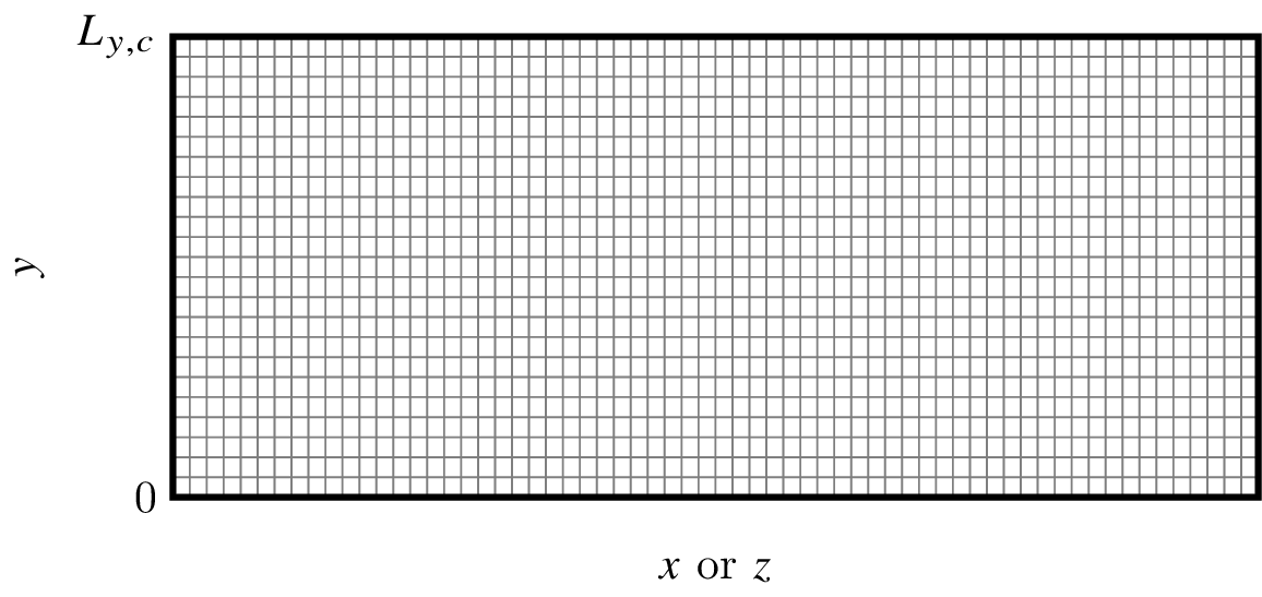 Figure 1: Example of the uniform grid type.
Stretched grid (wall-to-wall) (grid_type=1)
In this configuration, the grid spacing is non-uniform in the wall-normal (y) direction and is obtained by applying a hyperbolic tangent stretching to a uniformly distributed grid.
First, a uniformly spaced computational coordinate \(\eta \in [-1,1]\) is defined:
where:
- \(i = 1, \dots, N_y\) is the grid index
- \(N_y\) is the total number of grid points
Then, a stretching transformation is applied using a hyperbolic tangent function: where the parameters are the following:
where \(\alpha\) is the stretching parameter controlling grid clustering
- \(\alpha \rightarrow 0\): uniform grid (use
grid_type=0for uniform grids) - larger \(\alpha\): stronger clustering toward the walls
Finally, the stretched coordinate is shifted and scaled to match the physical domain size \([0, L_{y,c}]\):
The following variables can be set in the input parameters file:
| Variable | Corresponding input parameter | Default Value | Description |
|---|---|---|---|
| \(L_{y,c}\) | Ly_channel |
2 | Channel height |
| \(N_y\) | ny_global |
N/A | Total number of grid points in x |
| \(\alpha\) | alpha_stretch |
2.6 | Stretching factor |
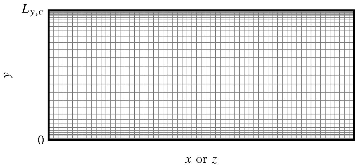 Figure 2: Example of the stretched grid type.
Stretched grid with uniform buffers on each end (grid_type=2)
In this configuration, the grid spacing in the wall-normal (y) direction is non-uniform in the center of the domain and uniform at the top and bottom of the domain. This grid type can be used in conjunction with, e.g., the standing_wave_x and traveling_wave_x body types to ensure that the grid spacing near the immersed boundaries is uniform (which is required for the IB method in this work).
The grid is centered about \(y = L_{y,c} / 2\) and is set up such that \(y = 0\) and \(y = L_{y,c}\) are the centers of the uniform regions. The total number of grid points (uniform and stretched regions combined) is \(N_y\). The stretching factor of the center region is set by \(\alpha\) in a similar to the stretched grid case. The width of the uniform buffers is controlled by the min_buffer_width input parameter. The code iteratively finds the grid spacing such that the width of the uniform region is at least as large as min_buffer_width plus twice the radius of the discrete delta function (see model and equations), while respecting the total number of grid points and the stretching factor.
The following input parameters are applicable:
| Variable | Corresponding input parameter | Default Value | Description |
|---|---|---|---|
| \(L_{y,c}\) | Ly_channel |
2 | Channel height |
| \(N_y\) | ny_global |
N/A | Total number of grid points in x |
| \(\alpha\) | alpha_stretch |
2.6 | Stretching factor |
min_buffer_width |
0.0 | Minimum buffer width |
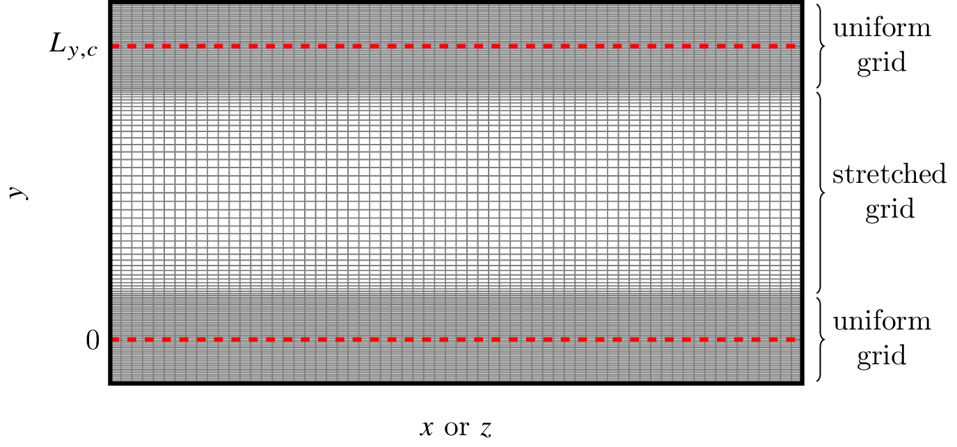 Figure 3: Example of the stretched grid type with uniform buffers.